Usage
This section describe an example usage of hiegeo.
Input files
For properly run hiegeo, you need two files:
- A .JSON file, that contains info about the discretization grid and the rendering of the plots.
- A data file (.CSV format) that include the actual data set, with information about the contact points, chronology and hierarchy.
JSON file
An example JSON file is provided in the file examples/hiegeo_test.json. It contains three main sections:
- colors
- This section contains the definition (HEX format) of the color that should be given to each SB. The color should be provided for the highest hierarchy SBs only.
- data_file
- The name of the CSV data file containing the data-set itself.
- grid
- Info about the grid used to discretize the domain. The notation should be straightforward.
CSV file
This file contains all the required information to create and plot SBs and SUs.
Its header should look like:
Apart from the very first column, that contains some index that are
used by the Python library pandas (but here they could be set to
whatever), the other columns content should be:
- gis_id
- This is simply a legacy column that contains the ID of the points extracted from the GIS software. You can set whatever value here as these are not used by hiegeo.
- chronology
- This is a very important column since it contains information about the chronology of the corresponding SB. The value should be an integer, that grows from the oldest to the youngest SB.
- hierarchy
- Another very important column, contains the hierarchy (sometimes called “rank”) of the SB. High level of hierarchy means high importance in sedimentary terms. In the provided example we have integer values ranging from 1 to 3.
- sb_name
- This is the name to be given to the SB. It should be a string
- su_name
- This is the name of the SU. Actually, this column is not implemented and the SU is named according to and internally consistent nomenclature.
- x
- The coordinate along the \(x\) axis of the (contact) points
- y
- The coordinate along the \(y\) axis of the (contact) points
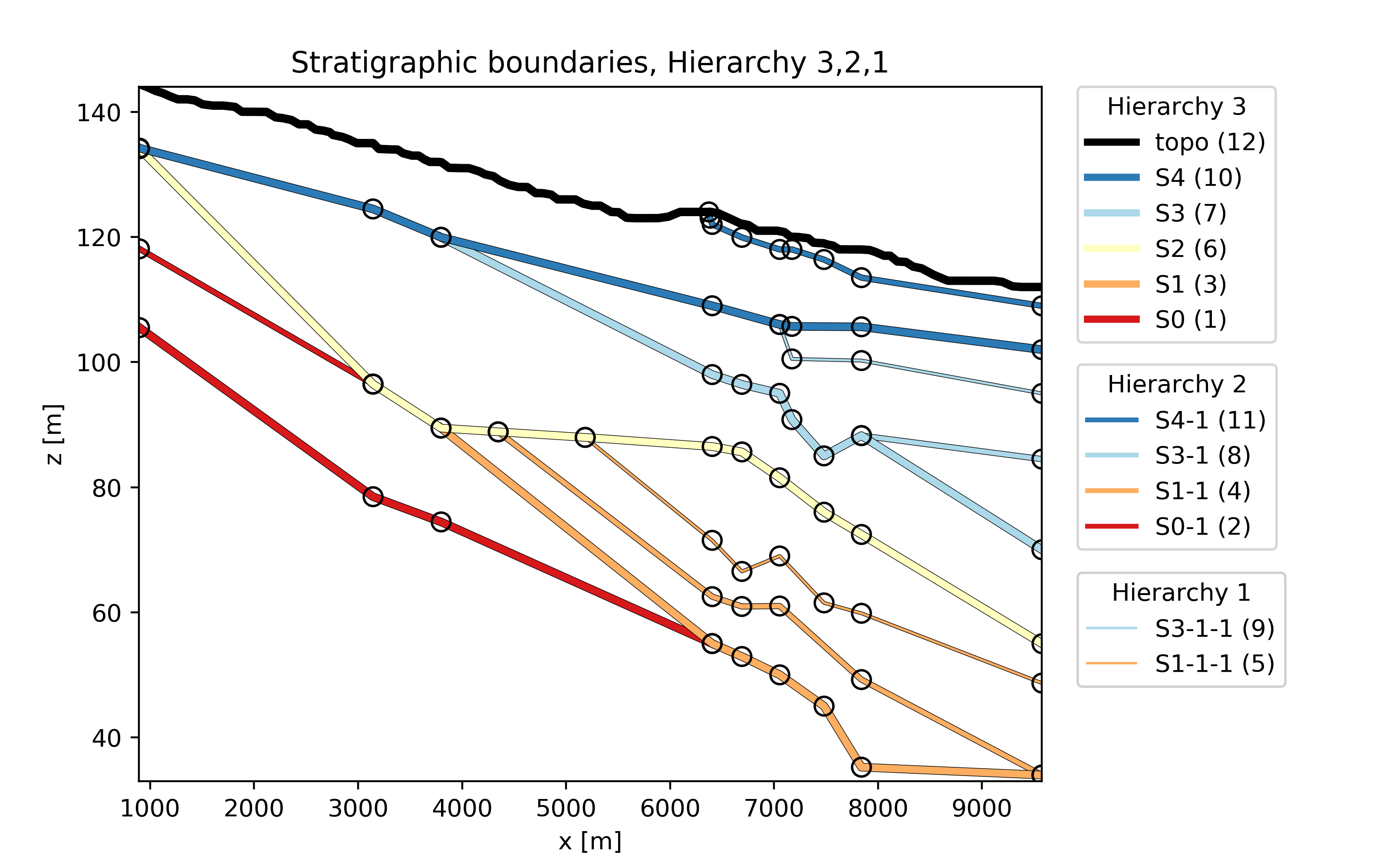
The following picture provides an illustration of the (subsurface) points contained in the data-set used for demonstrating the working principle of hiegeo.
Example scripts
Here two example scripts are provided in the examples folder. One file (hiegeo_test-simple.py) contains a full working example to read data, plot with a basic layout SBs and SUs, and provide a hierarchical representation of the geology with a tree structure. The other file, instead (hiegeo_test-full.py) provides a more complete example where plots are made for three different levels of hierarchical representation, with advanced plot legend and includes the creation of a GSLIB output file.
Both script should be sufficiently documented to allow running them without additional information.
You can move to the folder examples and there, from
the command line, run one of the two provided demonstration scripts.
For example:
./hiegeo_test-simple.py
and hit <Enter>. On Linux you will probably need to give execution rights to the file, like this:
chmod +x hiegeo_test-simple.py